Solar for IoT: A Practical Reference
July 14, 2026
Who this is for
This document is for someone building solar into a small connected outdoor device — maybe a battery-powered sensor you want to leave on a roof or in a field for a year without touching, a weather station, or a LoRa mesh repeater. You’re comfortable with basic electronics (you know what voltage and current are, you’ve probably built something with an Arduino or Raspberry Pi), but you haven’t designed power electronics before and you don’t have an engineering degree. The scope is small outdoor panels — roughly 100 milliwatts to 10 watts — powering devices with a microcontroller, a radio, some sensors, and a battery. The physics is the same as rooftop solar, but grid-tie inverters and utility connections are different problems. Indoor solar harvesting (powering a sensor from room lighting) is a related but distinct problem and isn’t covered.
By the end you should be able to:
- Read a solar cell datasheet and predict what it’ll actually deliver in your enclosure, not just on a lab bench.
- Size a solar cell and battery from a power budget without guessing.
- Pick a power-management chip that matches your scenario without it draining more than it harvests.
- Recognize the common failure modes before your prototype sits outside and dies in January.
The short version
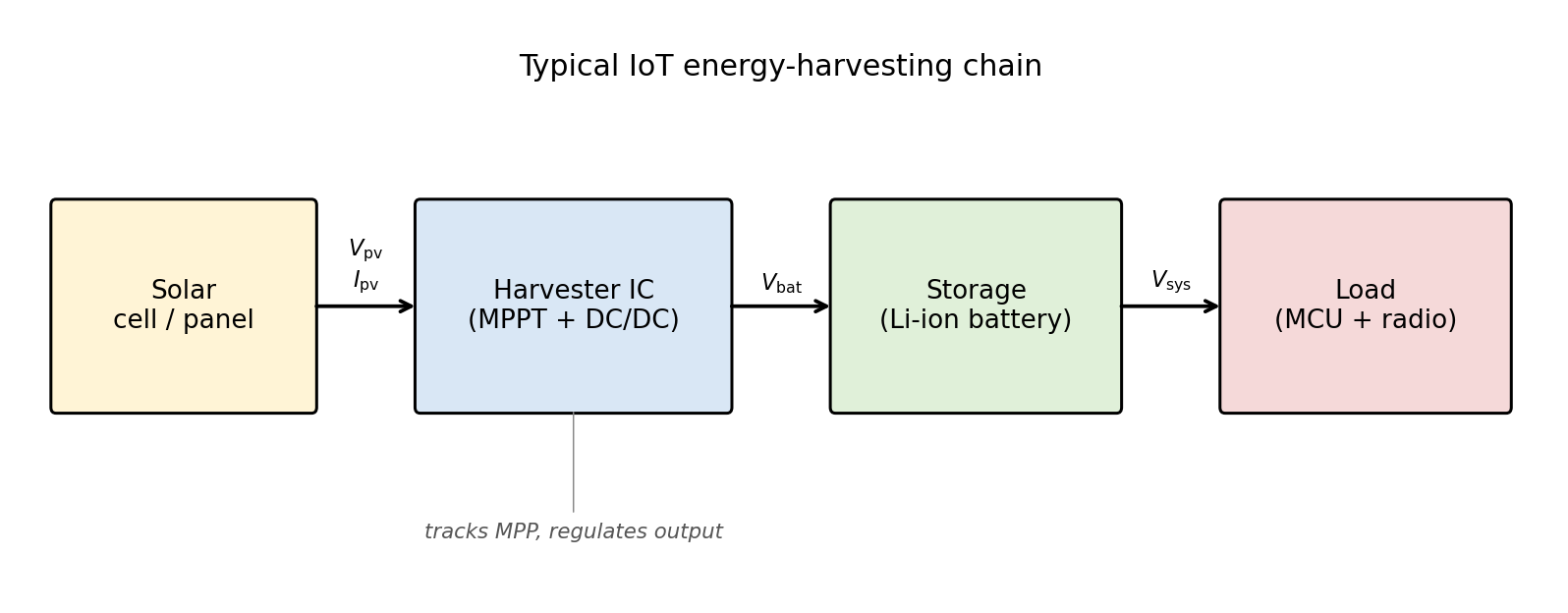
A solar-powered outdoor device is four parts in a line: a solar panel feeds a charger chip, which fills a battery, which runs your device. The panel only produces when the sun is out; the battery carries the device through nights and cloudy stretches. Almost everything hard about the design comes from three facts:
- The sun is unreliable. A panel’s rated wattage is a lab number you’ll rarely see outdoors, and winter delivers a fraction of summer. Size for the worst month, not the average, or it goes dark its first winter.
- The battery is fragile. Lithium cells are damaged by draining them flat and by charging them below freezing. Most of the parts list exists to protect the cell from those two things.
- A panel is not a battery. Its output voltage wanders with sunlight and temperature, so you can’t just wire it to a battery and expect good results. A small charger chip sits in between and does the matching.
Get those three right and the rest is arithmetic — which is most of what this document is, plus the physics behind it and the specific parts that do the work. There’s a glossary at the end for the acronyms.
You don’t need the physics to size a system. The next two sections explain why silicon behaves the way it does. If you just want to build, skip ahead to Sizing from a power budget and come back when you’re curious. If you’d rather see the whole process on a real device first, the Worked example near the end sizes a MeshCore repeater from scratch — some people read that first and refer back.
How a solar cell works
Silicon, the main ingredient in solar cells, is a semiconductor — a material that is neither a good conductor like copper nor a good insulator like glass, but somewhere in between. Pure silicon doesn’t do much electrically on its own. What makes it useful is doping: adding tiny amounts of other elements to change how its electrons behave.
Dope one piece of silicon with a little bit of phosphorus and you get n-type silicon, which has extra electrons floating around that can carry current. Dope another piece with a little boron and you get p-type silicon, which has “holes” — places where electrons are missing. Holes can also carry current; they behave like positive charges moving in the opposite direction to electrons.
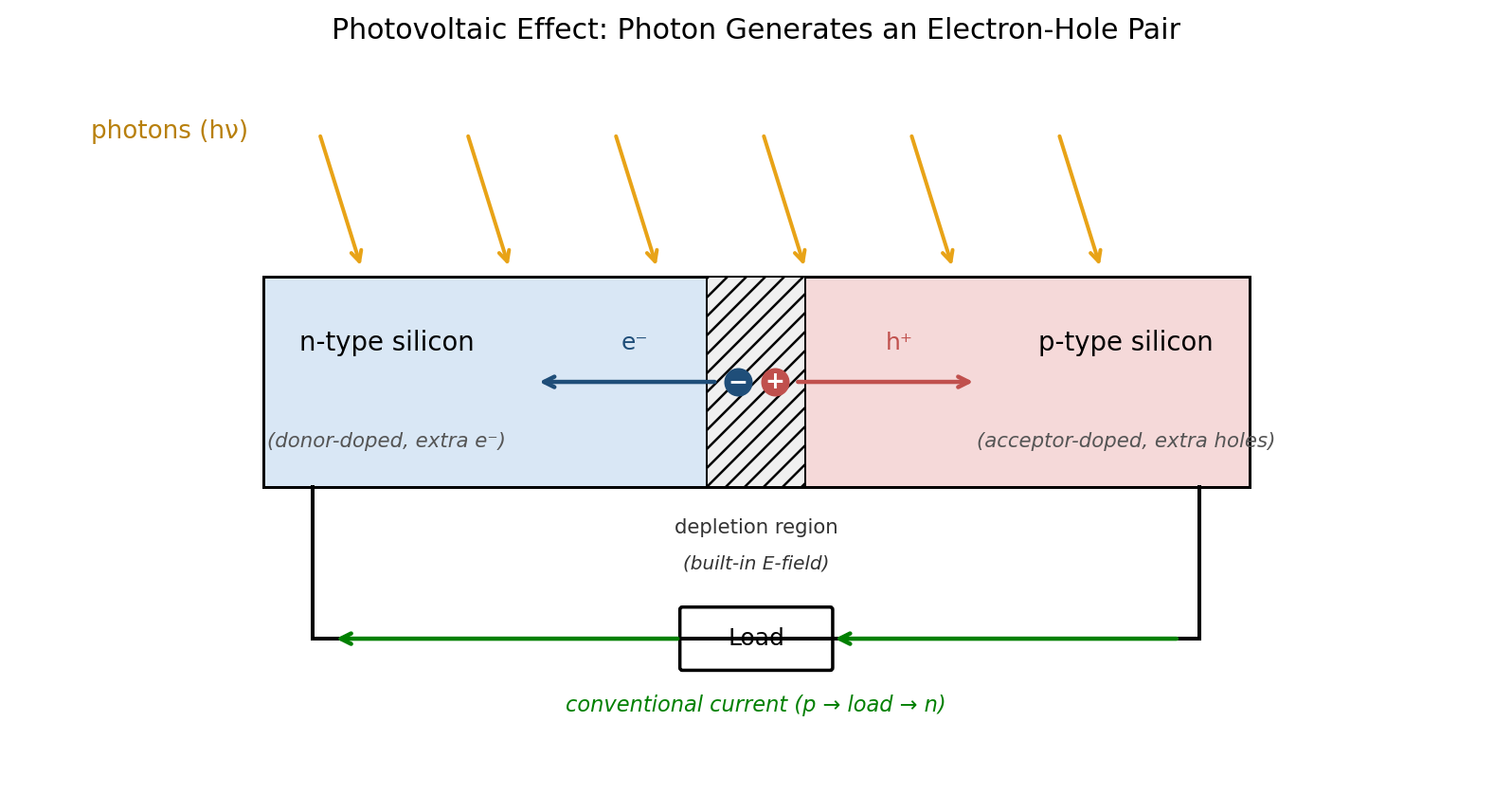
Now push an n-type piece and a p-type piece together. Near the boundary, the extra electrons from the n-side drift across and fill in the holes on the p-side, recombining. This leaves behind a thin layer — the depletion region — that has no free charges, just a built-in electric field pointing from n to p. That junction is what makes the device work.
When light hits the silicon, occasionally a photon (a little packet of light energy) gets absorbed and knocks an electron loose from an atom, leaving behind a fresh hole somewhere else. You now have a mobile electron-hole pair. If this happens near the depletion region, the built-in electric field grabs them and pulls them apart — the electron gets shoved toward the n-side, the hole toward the p-side. If you connect a wire from one side to the other, the electrons flow through the wire to get back to the holes on the other side. That flow is current, and you’ve just made electricity from sunlight.
Not every photon does useful work. Light is made of photons with different energies (different colors), and silicon only responds to photons with at least a certain minimum energy — called the bandgap. For silicon, the bandgap is about 1.1 electron-volts (eV), an energy unit common in physics. Red, green, and blue visible light all exceed this easily. Deep infrared photons don’t have enough energy and pass right through the cell doing nothing. On the other end, high-energy photons like blue and ultraviolet do get absorbed, but the excess energy over the bandgap is wasted as heat — the electron gets knocked loose and then immediately loses the extra energy before we can collect it.
Because of these losses plus a few others (reflection off the front surface, recombination inside the cell, resistance in the contacts), a single-junction silicon cell has a hard efficiency ceiling. The general thermodynamic limit for any single-junction cell — the Shockley-Queisser limit — is about 33% (roughly 32% at silicon’s 1.1 eV bandgap). Silicon then loses a bit more to an unavoidable process called Auger recombination, which pulls its true ceiling down to about 29%. The best commercial silicon cells today hit 23–25%, with record lab cells around 28%, closing in on that intrinsic limit.
The current-voltage (I-V) curve
If you take a solar cell sitting in constant light, connect it to a variable load, and slowly change the load from a dead short (zero resistance) to an open circuit (infinite resistance), you can measure the current flowing and the voltage across the cell at each setting. Plot current against voltage, and you get the cell’s I-V curve — the single most important diagram in solar design.
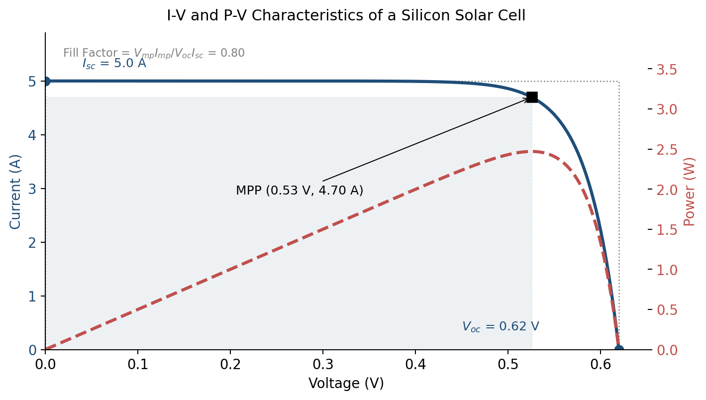
Three points on the curve matter, and you’ll see them referenced everywhere:
Short-circuit current (abbreviated \(I_{sc}\), the “sc” for short-circuit) is the current flowing when you short the terminals together with a wire — that is, when voltage is zero. It’s roughly proportional to how bright the light is: twice the light gives you twice the short-circuit current. This is the far-left end of the curve.
Open-circuit voltage (\(V_{oc}\)) is the voltage you measure across the terminals when nothing is connected, so no current flows. For a single silicon cell this is about 0.6 to 0.7 volts regardless of cell size. Interestingly, open-circuit voltage barely changes between bright sun and a dim cloudy day — it moves slowly (logarithmically) with light level. This is the far-right end of the curve.
Maximum power point (MPP) is the operating point where power — voltage times current — is largest. Since power is zero at both ends (no voltage at short-circuit, no current at open-circuit), there has to be a maximum somewhere in between. It’s at the “knee” of the curve, where the curve starts dropping steeply. This is where you want to operate the cell if you care about squeezing out the most energy.
There’s a summary number called the fill factor that tells you how “square” the curve is. If the curve were a perfect rectangle (full current all the way until suddenly dropping to zero at full voltage), the fill factor would be 1.0 — you’d be getting the theoretical maximum power. Real silicon cells have fill factors around 0.70 to 0.85, which is the ratio of the actual maximum power to the product of short-circuit current and open-circuit voltage. Higher is better.
Efficiency is what you might expect: the power you get out divided by the power of the sunlight falling on the cell. The reference condition for comparing cells is called Standard Test Conditions (STC): sunlight intensity of 1000 watts per square meter, cell temperature held at 25 °C, and a specific reference spectrum. Real outdoor sunlight is rarely at STC, which matters a lot — more on that below.
The crucial design insight from all this is that a solar cell is not a battery and not a constant-current source. It’s a nonlinear device where the best operating point depends on how bright the light is, how hot the cell is, and what else is happening. You can’t just connect a cell to a load and expect good results. You need something active sitting between the cell and whatever is being powered — a little electronic circuit that holds the cell at its maximum power point while delivering useful voltage to the battery. That circuit is called a power tracker, and we’ll get to it shortly.
From one cell to a panel
One silicon cell gives about 0.6 volts, regardless of whether it’s the size of a fingernail or a dinner plate. Area determines current instead — a bigger cell catches more photons and produces more current at that same voltage.
Most devices need more than 0.6 volts. The solution is to wire cells in series, which adds their voltages. Six cells in series gives about 3.6 volts (enough to charge a lithium battery through a converter); thirty-six cells in series gives about 21 V at open circuit and around 17–18 V at the maximum power point — that’s the classic “12-volt nominal” panel sized to charge lead-acid batteries with headroom; sixty or seventy-two cells in series gives roughly 36–49 volts (about 36–41 V for a 60-cell module, 44–49 V for 72-cell), which is what rooftop solar modules use.
Series wiring has a weakness worth knowing about: the current through a series string is only as good as the worst cell. If one cell in a 36-cell series panel is shaded, the whole panel’s current drops to whatever that shaded cell can supply, even though 35 other cells are in bright sun. Worse, the shaded cell gets pushed into a mode where it dissipates power as heat instead of generating it — which can create a damaging hot spot.
The standard fix is bypass diodes: extra diodes wired across sub-groups of cells (typically 10–24 cells per group). Normally they do nothing. But when a group gets shaded, the diode turns on and lets the healthy string’s current flow around the shaded group instead of through it. You lose that group’s output, but you don’t lose the whole panel and you don’t risk damage.
Temperature effects
Hot silicon cells produce less power than cold ones. This surprises people who expect solar cells to love hot sunny days. They do — sort of — but the extra sunlight only partly compensates for the temperature hit.
The three numbers to know, for typical silicon:
| What changes | Approximate coefficient | Meaning |
|---|---|---|
| Open-circuit voltage | drops 0.3% per °C | Main reason hot cells lose power |
| Short-circuit current | rises 0.05% per °C | Small benefit that doesn’t offset the loss |
| Maximum power | drops 0.4% per °C | Net effect on output |
A cell sitting in direct sun typically ends up 20–30 °C hotter than the surrounding air because it absorbs more light than it converts. So a 35 °C ambient day can put the cell at 60 °C, which knocks its output down about 14% from the STC-rated value. That’s why panel datasheets always quote two sets of numbers: STC (optimistic, rarely seen in real life) and NOCT, “Nominal Operating Cell Temperature” (more realistic).
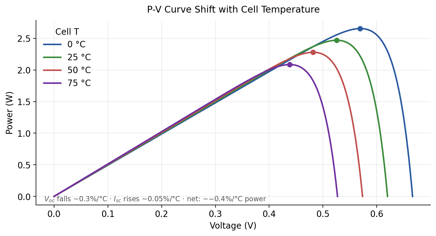
Notice that as the cell heats up, the peak of the curve moves to the left — toward lower voltages. This is why a “set it and forget it” fixed-voltage charger will slowly lose efficiency through the day as the cell warms up. A real power tracker follows the knee around as it moves.
Why you need a power tracker
Here’s the problem with just wiring a solar cell directly to a battery. Suppose you have a small panel whose open-circuit voltage is 6 volts and whose maximum-power-point voltage (where it produces the most power) is around 4.8 volts. You want to charge a 3.7-volt lithium battery. Connect them directly.
The battery’s voltage is roughly fixed at 3.7 volts (that’s how batteries work — they don’t let their voltage stray far from their chemistry’s set point). So even though the panel would prefer to operate at 4.8 volts, the battery drags it down to 3.7. Looking back at the I-V curve, operating far from the knee means you’re getting nearly full current but much less voltage than optimal. Since power is voltage times current, you might end up harvesting only about 40% of the power the panel could deliver. That’s a lot of free energy left on the table.
A maximum power point tracker (MPPT) is a small circuit that sits between the panel and the battery. It’s a type of DC-DC converter, which means it transforms one DC voltage into another (like how a transformer does for AC). The MPPT version has a control loop that constantly adjusts things to hold the panel at its best operating point, while converting whatever voltage that is into whatever the battery needs.
The simplest MPPT algorithm is called perturb-and-observe: nudge the operating voltage a little, measure whether power went up or down, and then keep nudging in the direction that helps. When you overshoot the peak, power drops and the algorithm reverses. Done continuously, this keeps the panel on its knee no matter how the light or temperature shifts.
For rooftop solar, the MPPT converter is a separate piece of hardware with its own microcontroller. For battery-powered gadgets, the same function lives inside a single integrated circuit that draws only a few hundred nanoamps when idle and can start up from less than a volt of input. That’s the subject of a section below.
A quick note on PWM. You’ll see “PWM” charge controllers mentioned in 12 V RV and off-grid solar discussions. PWM is a simpler, cheaper alternative that rapidly switches the panel on and off to regulate charging voltage. The catch: it clamps the panel’s operating voltage to battery voltage, which throws away all the power the panel could have delivered at voltages above that. It works acceptably when panel and battery voltages are closely matched (a nominal 12 V panel into a 12 V lead-acid battery) but loses 20–25% in most other cases. All the chips in this document do MPPT; PWM is rare below 50 W standalone controllers.
Choosing a cell for outdoor use
For outdoor deployments, the choice is almost always between monocrystalline and polycrystalline silicon. Both are the same underlying technology; they differ in how the silicon is grown, which changes efficiency, cost, and appearance.
| Technology | Efficiency | Typical look | Best use case |
|---|---|---|---|
| Monocrystalline silicon | 18–24% | Dark, uniform, often cut with chamfered corners | Compact, best efficiency per area |
| Polycrystalline silicon | 15–18% | Speckled blue, squarish cells | Cheaper per watt, slightly bulkier |
Monocrystalline is the usual pick for small outdoor IoT panels. The efficiency advantage matters more when panel area is constrained — a 100 × 100 mm mono panel produces about 25% more power than the same-sized poly panel. For a 5 W panel destined for a rooftop LoRa node, that’s the difference between 5 W and 4 W, which can add up to a meaningful reliability margin in bad months. Poly costs less per watt but is bulkier for the same output, and mono is now the default even for large fixed installations.
The exotic technologies you’ll see mentioned in solar literature — amorphous silicon, gallium arsenide, dye-sensitized cells, organic photovoltaic — are mostly optimized for indoor artificial light, where their spectral response is a better match than crystalline silicon. For outdoor use they’re either less efficient (amorphous, DSSC, OPV) or far more expensive (GaAs) than crystalline silicon. Skip them unless you have a specific reason not to.
Outdoor irradiance varies much more than people expect
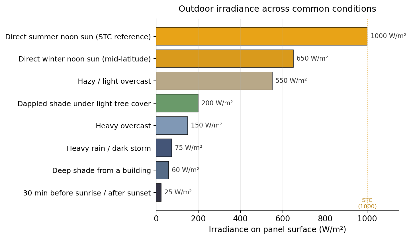
Panel specifications quote power at Standard Test Conditions (STC): 1000 W/m², 25 °C, specific reference spectrum. Real outdoor conditions are rarely at STC, and the variation is larger than most people intuit.
A few takeaways for design:
- Winter sun is weaker even when the sky is clear, because the sun is lower in the sky and light passes through more atmosphere. At 35° N latitude, noon-sun irradiance on a horizontal surface in December runs 30-40% below the summer peak even on a cloudless day — only about 15-20% of that is the extra atmosphere the low sun shoots through; the rest is the shallow angle onto a flat surface, much of which you recover by tilting the panel toward the winter sun (see mounting, below). This is on top of the shorter day length, compounding the winter shortfall.
- Overcast is much darker than it looks. Thick cloud cover drops irradiance to 10-20% of clear-sky values. Our eyes adjust, but the panel doesn’t care how bright things seem subjectively.
- Shade from nearby objects is almost entirely diffuse sky light at 5-10% of direct sun. A panel in the deep shadow of a building can produce twenty times less power than one in direct sun right next to it.
This variation is why the worst-month peak-sun-hours number (covered later) matters so much for reliable outdoor deployments.
Sizing from a power budget
Before picking a panel, work out how much energy the device actually needs. The process is mechanical — essentially a list of numbers that get multiplied and divided — which is how it should be.
Step 1 — Work out average power. Most battery-powered devices spend most of their time asleep, waking briefly to take a reading or transmit. So the average power is the sum of sleep power (tiny, but constant) and active power (large, but only for brief moments).
If the device wakes for 10 milliseconds at 10 milliamps and 3 volts once per minute, and sleeps at 2 microamps the rest of the time, then:
- Energy per wake event: 10 ms × 10 mA × 3 V = 0.3 millijoules
- One wake event per 60 seconds, so average active power: 0.3 mJ / 60 s = 5 microwatts
- Sleep power: 2 microamps × 3 V = 6 microwatts
- Average total: about 11 microwatts
Step 2 — Multiply by a day to get daily energy. Eleven microwatts times 86 400 seconds in a day is about 0.95 joules, or 0.26 milliwatt-hours. That’s the energy the device needs to collect every day to stay alive indefinitely.
Step 3 — Convert daily energy to required panel size using “peak sun hours.” Peak sun hours (PSH) is a useful cheat: the number of hours per day equivalent to full 1000 W/m² sunlight. So 4 PSH means “the day delivers the same total energy as 4 hours of bright noon sun.” PSH varies with season and location; for a temperate mid-latitude climate, annual average is around 4–5, and the worst month (December in the northern hemisphere) is closer to 2.5. (That 2.5 is a conservative flat-panel figure; a panel tilted toward the winter sun can see 3.5–5 PSH even in December at these latitudes, so designing around 2.5 bakes in extra margin.) Always design around the worst month unless the battery is huge enough to ride through bad stretches.
Required panel output (at STC) = daily energy / (peak sun hours × harvest efficiency). If daily energy is 0.26 mWh, PSH is 2.5, and you assume your whole chain is 40% efficient, then the panel needs to be rated for about 0.26 milliwatts at STC — which after rounding up becomes a tiny panel indeed.
Step 4 — Derate aggressively. STC ratings are lab-condition numbers. Real deployments take hits from:
- The power-management chip (70–90% efficient)
- The battery (90–95% round-trip efficient)
- Dust and dirt on the panel (3–10% loss)
- Panel angle not being optimal (5–20% loss)
- Aging over 20 years (up to 20% loss at end of life)
- Heat (5–20% loss on hot days — or use the NOCT figure from the datasheet if available, which bakes in a realistic cell temperature)
Multiply all these together and you end up at about 35–60% of the nameplate number. A 1-watt panel is really a 400-milliwatt panel in practice.
Step 5 — Size the battery for the worst dark stretch you expect. For outdoor deployments in most climates, plan for 3 to 7 cloudy or rainy days in a row where you’ll get almost nothing from the panel. The battery needs to hold enough energy to keep the device running through that stretch on its own.
Battery chemistry
Lithium-ion (Li-ion) and its polymer variant (LiPo) are the default choice for small outdoor solar IoT. They have the highest energy density (the most watt-hours per gram and per cubic centimeter) of any readily-available rechargeable chemistry, widely available cells in every form factor from coin cells to 18650 cylinders to custom pouch cells, and charge management ICs designed for them. When someone says “the battery” in an IoT context, they almost always mean Li-ion.
Key properties of a typical Li-ion cell:
- Voltage: 3.0 V discharged, 4.2 V fully charged, 3.7 V nominal average.
- Energy density: 250–700 Wh/L, 150–250 Wh/kg.
- Cycle life: 300–1000 full charge cycles before capacity drops noticeably.
- Calendar life: 2–5 years before capacity fade becomes limiting, even without cycling.
- Charge temperature range: 0 to 45 °C (with important caveats covered in the next section).
- Self-discharge: 2–5% per month when idle.
- Round-trip energy efficiency: 90–95%. (The coulombic charge efficiency — charge out versus in — is itself above 99%; the few-percent loss is mostly the voltage gap between charging and discharging.)
Alternatives worth knowing about
Two other lithium chemistries show up often enough to know about. LiFePO4 (lithium iron phosphate) trades some energy density for a much longer cycle life (2000–5000 cycles) and better tolerance of cold charging. Cell voltage is lower — 3.2 V nominal versus 3.7 V for Li-ion — which matters if your device expects a Li-ion voltage range. Worth it for cold climates or decade-long deployments. LTO (lithium titanate) is the extreme-environment option: safe to charge down to −30 °C, 10 000+ cycles, but costs more and has lower energy density. Worth the tradeoffs for mission-critical remote nodes.
For the rest of this document, “battery” means Li-ion unless otherwise stated.
Safe charging rates (C-rate)
Battery charge and discharge speeds are usually expressed as a multiple of the battery’s capacity, written “C.” The rule is simple: charging current (in amps) equals battery capacity (in amp-hours) times the C-rate. So charging a 2000 mAh (2 Ah) battery at 0.5C means 1 amp of charging current; at 1C, 2 amps; at 0.1C, 200 milliamps. The charge rate also tells you roughly how long a full charge takes — 1C fills the battery in about an hour, 0.5C in two hours, 0.1C in ten hours.
Faster charging stresses the cell more. Every lithium cell has a maximum charge rate listed in its datasheet, and the broad manufacturer advice from sources like Battery University converges on a few numbers:
- 0.5C is best for longevity. Cells charged at this rate can deliver significantly more cycles than the same cells charged at 1C.
- 1C is the safe default. Virtually all modern Li-ion and LiPo cells tolerate this, and it’s what most consumer devices do.
- Above 1C only if the datasheet explicitly allows. Drone and RC battery packs often allow 2C or higher, but most generic cells don’t.
For small solar IoT, you almost always land well below these limits without trying. A 1-watt panel feeding a 2000 mAh Li-ion battery maxes out at around 300 milliamps of charging current (panel power divided by battery voltage, roughly), which is 0.15C — below the “longevity-friendly” 0.5C number. Bigger batteries or smaller panels push this even lower. At typical small-panel IoT scales, you’re naturally in the gentle-charging regime, and you don’t really need to worry about C-rate unless you’ve paired a small battery with an unusually large panel.
Charging in the cold
Below about 0 °C (32 °F) the conventional advice is sharp: don’t charge Li-ion or LiPo at all. The mechanism is well-understood. When lithium ions arrive at the anode faster than the cold, sluggish electrolyte can absorb them into the graphite structure, they plate out as metallic lithium on the surface instead. That plating is permanent — it reduces capacity, raises internal resistance, and in the worst case grows into dendrites that can puncture the separator between anode and cathode, causing an internal short. LiFePO4 tolerates cold charging somewhat better (down to about −10 °C for some cells) but isn’t immune.
Here’s where the conventional rule deserves more nuance, though. The “don’t charge below freezing” advice is calibrated for the charge rates consumer electronics use: 0.5C to 2C for a phone or laptop, up to several C for fast-charging EVs. At those rates, plating below freezing is a fast and real problem. But the research literature (cited by Battery University) puts the theoretical safe cold-charge rate at −30 °C at about 0.02C. That’s a 50-hour charge time for a standard cell, which is why it’s usually dismissed as impractical — but it’s still safe.
The implication for small-panel IoT is significant. If your worst-case charge rate is already 0.05C or 0.1C (easy to arrive at with a 1 W panel into a 3000 mAh cell), you’re operating near or at the published theoretical cold-safe rate. Field experience backs this up. The YYCMesh community has run dozens of nRF52-based LoRa mesh nodes through two full Canadian Rockies winters, occasionally hitting −40 °C, with charge rates held under 0.1C the whole time. They report about 6% capacity loss — well within spec — and internal resistance still within factory spec after two years of service. This doesn’t mean cold-charging is safe in general — but it does mean the blanket “never below 0 °C” rule is overcautious for this specific regime. The real pitfall is high-rate cold charging, not cold charging as a category.
Practical takeaways for cold-climate solar IoT:
- Size the panel and battery so the worst-case charge rate stays below 0.1C. For most small-panel designs this is automatic, but check the math — it’s just panel wattage divided by battery voltage divided by battery capacity.
- Don’t rely on a low-temperature charge-cutoff as your only defense. If the cutoff is set at 0 °C, a long cold snap leaves the device dead with no way to recharge even at safe low rates. A more forgiving cutoff (or none at all, paired with a low charge rate by design) often serves better.
- Consider LiFePO4 for extreme cold climates. It tolerates cold charging somewhat better than Li-ion and has a longer cycle life, at the cost of lower energy density. Only worth the tradeoff if you’re deploying somewhere that reliably hits deep-cold temperatures for weeks at a time.
- When in doubt, measure. A panel-voltage log and a battery-temperature log from one full winter tell you more than any theoretical calculation.
Protecting against over-discharge
A lithium-ion cell discharged too deeply — below about 3.0 V per cell for standard Li-ion, 2.5 V for LiFePO4 — sustains permanent damage. The anode starts to dissolve into the electrolyte, and on the next charge cycle the cell ends up with reduced capacity and higher internal resistance. Push it further (below about 2.5 V for Li-ion) and the cell may fail to charge at all. For a rooftop solar node that accidentally runs its battery flat during a long dark stretch, this is a one-strike event — the battery is damaged before anyone notices.
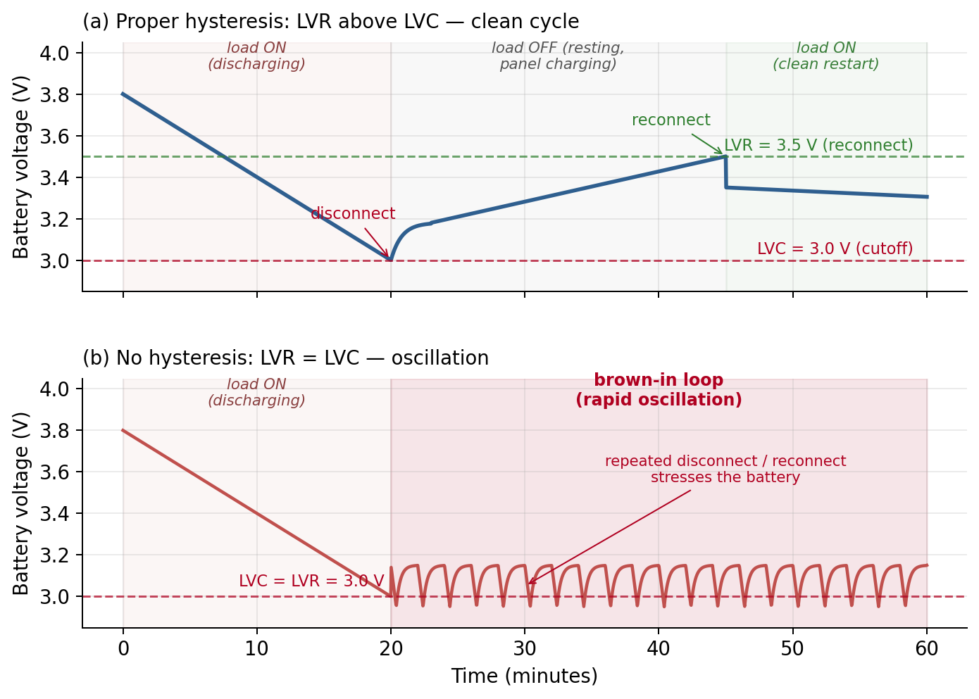
The standard defense is a low-voltage cutoff (LVC) — a threshold voltage at which the load disconnects from the battery. But just having a cutoff isn’t quite enough. Once the load disconnects, the battery’s resting voltage recovers as the internal resistance drop disappears — a battery at 2.95 V under load might sit at 3.10 V with no load. If the reconnect threshold is the same as the cutoff, the device boots up, starts drawing current, sags immediately back below the cutoff, disconnects, recovers, boots again, and cycles. This “brown-in loop” can hammer a weak battery harder than a clean shutdown would have, because each boot cycle pulls meaningful current through MCU startup, radio init, and any sensor warm-up.
The fix is hysteresis: a low-voltage reconnect (LVR) threshold set well above the cutoff. Typical values:
| Chemistry | Cutoff (LVC) | Reconnect (LVR) |
|---|---|---|
| Li-ion / LiPo | 3.0 V | 3.4–3.6 V |
| LiFePO4 | 2.5 V | 3.0–3.2 V |
| LTO | 1.5 V | 2.0–2.2 V |
The reconnect threshold should be high enough that when the device boots and loads the battery, the voltage under load stays comfortably above the cutoff. Bigger gap means longer to come back online after a deep discharge, but less battery abuse.
Three places this protection can live, from outside to inside:
- On the battery itself. Protected 18650 cells have a small protection circuit module (PCM) built in that disconnects at around 2.5 V and reconnects at around 3.0 V. Cheap and automatic, but the thresholds are fixed and often not ideal. Unprotected cells have no built-in cutoff at all.
- In the harvester or charger chip. Most chips in the earlier PMIC tables have a UVLO (undervoltage lockout) that disables their output below some voltage. On the BQ25570 this is set by a resistor divider, typically at 2.2–3.0 V.
- In firmware. The MCU reads battery voltage through an ADC and decides whether to keep running or shut down. Most flexible — you can implement multiple thresholds (reduce TX power below X, stop transmitting below Y, shut down below Z) — but it requires the device to actually be running, so it can’t protect the “already offline” case.
Concrete example: MeshCore “voltage bootlock.” Immediately after boot and before any mesh operations start, the firmware reads battery voltage. If the voltage is below a configurable threshold (3.3 V by default), the firmware configures the nRF52’s low-power comparator to wake the device only when battery voltage rises above a recovery threshold (or USB power is applied), then enters SYSTEMOFF. This prevents the boot-sag-shutdown loop even when the PMIC’s UVLO is set too low. For solar nodes that routinely see deep discharge through long dark stretches, firmware-level protection like this is worth having — the harvester chip’s UVLO is often set low to maximize runtime and leaves no headroom for the boot surge.
Design rules of thumb:
- Always have an LVC. No exceptions — the cutoff protects the cell itself.
- Add an LVR with at least 400 mV of hysteresis for Li-ion. Less than that risks brown-in loops.
- Layer the protection. Battery PCM + harvester UVLO + firmware check. Any one can fail or be mis-set; the others catch it.
- If your firmware supports it, use it. A software bootlock complements the hardware UVLO rather than replacing it.
Power-management chips for small devices
This is where battery-powered solar diverges sharply from rooftop solar. You can’t use a big MPPT converter — it would be idle most of the time, and its own idling current consumption would swallow everything the cell collects. The chips available for small-scale solar fall into two broad classes based on how much power you need to harvest.
Which chip class to use
- Average load under a milliwatt, panel under 100 mW: use a micropower harvester like the TI BQ25570. These chips cold-start from sub-volt inputs and idle in the nanoampere range, so they can power a duty-cycled BLE sensor or indoor-adjacent outdoor node without self-defeating overhead.
- Average load between 10 mW and several watts, panel in the 1–10 W range: use a watt-scale chip like the Consonance CN3791 or ADI LT3652. These expect several volts of input and milliamp-to-amp charging currents. The typical MeshCore repeater, ESP32 weather station, or small Raspberry Pi Zero node lands here.
- Load bigger than that: you’re looking at a dedicated solar charge controller (Victron, Genasun, and so on), not an IC, which is outside the scope of this document.
The rest of this section covers both chip classes in detail, starting with the micropower family.
Micropower harvester chips
Micropower harvester chips are designed for the sub-milliwatt world. Two specs matter most:
- Cold-start voltage: the minimum input voltage needed to boot the chip up from a dead battery. Lower is better because it means the chip can wake up from dim light.
- Quiescent current: how much current the chip itself draws when idling. Measured in nanoamps (billionths of an amp) for the best ones. Every nanoamp the chip consumes is a nanoamp your battery doesn’t get.
A few popular parts:
| Chip | MPPT method | Minimum cold-start input | Idle current | Notes |
|---|---|---|---|---|
| TI BQ25570 | FOCV (see below) | 600 mV | about 488 nA | Both boost and buck, battery-aware |
| TI BQ25504 | FOCV | 600 mV | about 330 nA | Boost only |
| E-peas AEM10941 | Custom | 380 mV | about 400 nA | 4 ratios: 70/75/85/90% |
| ST SPV1050 | FOCV | 550 mV | about 2.5 microamps | Boost or buck-boost |
| ADI ADP5091/2 | FOCV (dynamic) | 380 mV | about 390 nA | Bursty regulation style |
| E-peas AEM30330 | MPPT | 275 mV | about 50 nA | Small PV, plus heat and RF sources |
Once running, most of these can keep harvesting from even lower input voltages (around 100 mV) — the cold-start number is only the barrier to bootstrap.
A clever shortcut: FOCV
For big rooftop systems, perturb-and-observe (the “nudge and measure” algorithm described earlier) tracks the maximum power point to within about 1% of the true peak. The catch: running that loop constantly costs power. At rooftop scales that’s negligible, but at micropower scales the algorithm’s own overhead can eat a noticeable slice of your harvest.
There’s a useful shortcut called fractional open-circuit voltage (FOCV). Empirically, for silicon cells, the maximum power point voltage always lands at roughly 76–82% of the open-circuit voltage, almost regardless of how bright the light is or how hot the cell is. So instead of continuously searching for the peak, the chip periodically does this:
- Disconnect the panel from the load for a few milliseconds.
- While disconnected, measure the open-circuit voltage (easy — just read an ADC).
- Set the operating point to about 80% of that measured voltage.
- Reconnect and run there until the next check, typically 16 to 64 seconds later.
This gets you within 95–98% of the true maximum power point with nearly zero continuous overhead. For tiny harvesters, that’s the better trade. The BQ25570 uses this by default, and the ratio (70% to 80% per its datasheet) is set by an external resistor divider.
Scaling up: when the panel is watts, not milliwatts
For panels in the 1–10 W range feeding bigger loads (a Raspberry Pi, an ESP32 with cellular, a small camera), a different class of chip takes over. The most common example on hobbyist boards is the Consonance CN3791, which appears on dozens of cheap breakout modules sold for 6 V, 9 V, 12 V, and 18 V solar panels. Two close relatives are worth knowing about: the CN3722 (same chip family, multi-cell) and the LT3652 (premium alternative).
| Chip | MPPT method | Input range | Idle / shutdown current | Charge current | Notes |
|---|---|---|---|---|---|
| Consonance CN3791 | Fixed voltage (constant-V) | ~4.5 V to ~28 V, must exceed \(V_{bat}\) | ~9 µA IC (~30 µA on a breakout) | up to 4 A | Single-cell Li-ion; needs external P-MOSFET + inductor; ~$0.50 chip, $3–10 breakout |
| Consonance CN3722 | Fixed voltage (constant-V) | ~7.5 V to ~28 V | similar to CN3791 | up to 5 A | 2S/3S/4S Li-ion and LiFePO4 stacks; otherwise same family as CN3791 |
| ADI LT3652 | Fixed voltage (constant-V) | 4.95 V to 32 V (34 V on HV; 40 V abs max) | 85 µA standby, 15 µA shutdown | up to 2 A | Multi-chemistry (Li-ion, LiFePO4, NiMH, lead-acid); monolithic (no external MOSFET); NTC battery-temp input; ~$8 chip, $27+ breakout |
All three use the same simpler MPPT approach: instead of continuously re-measuring open-circuit voltage like the micropower harvesters do (true FOCV), you pre-configure a single fixed panel voltage via an external resistor divider — “hold the panel at about 5 V” for a 6 V panel, for example. The key distinction from true FOCV is that the target is set once at design time and never updates — it doesn’t adjust for temperature or cell aging. This works because a silicon panel’s maximum-power-point voltage is nearly constant as irradiance changes and shifts only slowly with temperature. You give up a few percent of harvest efficiency versus true FOCV in exchange for dead-simple hardware.
Pick between them based on battery stack and budget. The CN3791 is the default for single-cell Li-ion — cheap, well-documented in the hobbyist community, works fine. The CN3722 is its multi-cell sibling: same constant-voltage MPPT, same parts-bin tier, but charges 2S/3S/4S Li-ion or LiFePO4 stacks. Reach for it when your load needs 7.4 V or 12 V system voltage without a separate boost stage. The LT3652 is the premium option: ten to twenty times the chip price, but it’s monolithic (no external MOSFET means a cleaner board and smaller footprint), supports essentially every rechargeable chemistry including NiMH and lead-acid, includes a battery-temperature input for safe cold-weather charging, and comes with the kind of silicon quality and application-note support that the Chinese parts don’t offer. Worth it if you’re building something production-grade, if multi-chemistry flexibility matters, or if space is tight.
The 30 µA sleep current and 4 V minimum input on the CN3791 would be disqualifying in a BLE sensor design, but they’re fine here. The sleep draw is tiny compared to the battery (a 2000 mAh cell lasts roughly 8 years on 30 µA), and anything running a Raspberry Pi has a panel big enough to provide several volts without effort.
Reverse-leakage protection
Here’s a subtle problem. A solar cell is a diode; in the dark, if you apply voltage to it from the wrong side, it conducts and drains whatever is connected to it. So a panel wired straight to a battery will slowly leak the battery’s charge through itself at night. This is small but not zero, and over months it matters.
There are three standard fixes:
- A Schottky diode in series with the panel. Simplest and cheapest. Schottky diodes drop about 200 millivolts when forward-conducting. That’s fine for larger systems but a showstopper for low-voltage harvesters where 200 mV is a big chunk of your headroom.
- An “ideal-diode” controller (parts like LTC4411 or MAX40200). These use a MOSFET and some control logic to behave like a diode but with a much smaller drop — tens of millivolts at light loads, rising to about 0.14 V near 1 amp — and very low idle current.
- Let the harvester chip handle it internally. Most modern chips — the BQ25570, the CN3791, the LT3652, and essentially everything else in the tables above — have built-in reverse-current blocking — the panel-direction leakage runs from tens of nanoamps in the best harvesters up to a few microamps in the simpler ideal-diode parts. When input voltage drops below battery voltage, the chip turns off its pass element and enters sleep mode, pulling a small idle current from the battery rather than letting it leak backwards through the panel.
If the harvester chip already handles reverse current (and most do), you don’t need anything else. If it doesn’t, an ideal-diode controller is usually the right answer; use a Schottky only when headroom isn’t tight.
Temperature, placement, and mounting
Cells get hotter than the air around them
A panel lying flat against a black plastic enclosure in direct sun can run 40 °C hotter than the air. Two almost-free fixes:
- Put a small air gap behind the panel. Even 5 millimeters of standoff with both ends open lets air flow and can drop cell temperature by 10–15 °C.
- Use a light-colored enclosure instead of black, especially if the enclosure physically touches the panel.
Angle is less important than you’d think
For a fixed panel in the northern hemisphere, the classic rule for maximum annual energy is “tilt the panel at an angle equal to your latitude, facing south.” But for battery-backed devices, you often care about the worst month (usually December) more than the total annual energy, which means tilting steeper — more like latitude plus 15°. If the enclosure forces you to mount the panel flat on top of something, you lose about 10–15% annually at mid-latitudes. Usually acceptable.
Outdoor enclosure reality check
- Encapsulation: Raw cells delaminate outdoors within a year. Use panels that are epoxy-encapsulated or ETFE-laminated (two types of weatherproof coating).
- Connectors: Use waterproof IP67 or IP68 rated connectors between the panel and enclosure. Small JST connectors for low current, MC4 connectors for higher current. Strain-relieve the cable or it will fatigue at the solder joint over seasons.
- Plastic choice: Polycarbonate holds up outdoors for years. ABS plastic starts yellowing within weeks and turns brittle and cracks over 1–2 years. PLA is not a material for outdoor use.
- Wildlife: Squirrels chew silicone cable jackets. If you’re in rodent country, use braided steel sleeving over the cable.
Shading and partial light
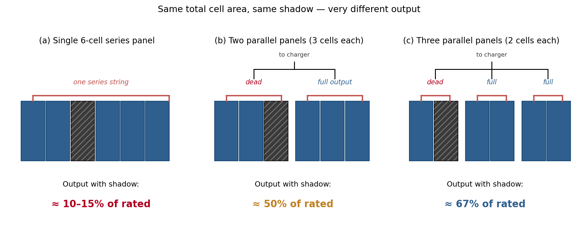
Shading is the single most common cause of outdoor solar deployments underperforming, and it deserves more attention than it usually gets. The core issue: series-wired cells are only as strong as their weakest cell. On a panel where cells are wired in series (most commercial panels), a single leaf or pigeon dropping covering one cell can drop total output by 50% or more — far worse than proportional to the shaded area. The shaded cell’s current becomes the bottleneck for the entire string. The same effect applies to multiple panels wired in series.
How shading shows up in the field
Shadows aren’t just “full shade” or “full sun.” Partial shade — diffuse, dappled, or moving — is where the real losses hide. A few patterns cost more output than people expect:
- A stationary shadow stripe from a fixed obstruction (flagpole, antenna, tree trunk). At the same time every day, a narrow shadow crosses the panel. If it hits different cells at different times on a series-wired panel, each sweep is a serious output drop.
- Uneven soiling — dirt or bird droppings on some cells but not others. A patch of dirt covering 10% of a panel can cost 40% or more of output.
- Tree shade filtering through branches. Even partial overhead foliage can cut output dramatically because the shade is spotty and moves with the sun and wind.
- Building edges at low sun angles. A nearby wall that looks clear at noon might cast a morning or afternoon shadow across the panel for hours, and the problem is worst in winter when the sun is lowest.
Multiple small panels beat one big panel (when shade is a risk)
The most effective shade mitigation for small outdoor deployments is to split the panel budget across two or more smaller panels mounted in different positions, wired in parallel. This has several advantages:
- A shadow over one panel doesn’t kill the others. Unshaded panels keep producing near their normal output. With one large panel, the same shadow can take out the whole thing.
- You can diversify the panel orientations. One panel facing east and one facing west captures more total energy across a day than two south-facing panels — the east panel picks up morning sun the south-facing pair would miss, and similarly for afternoon. Peak output is lower, but the day’s total energy is often higher, which matters most when the battery is smaller than a day’s energy.
- A partial failure isn’t a total failure. If a connector corrodes or a panel delaminates, you lose one panel’s share, not all of it.
When wiring panels in parallel, a diode in series with each panel’s positive lead prevents current flowing backwards from unshaded panels into shaded ones — without it, a shaded panel can become a load on its brighter neighbors, burning off power instead of generating it. This is genuinely worth doing when the panels diverge in orientation or shading (as in the drone-detector build later); it’s more debatable for identical, similarly-aimed panels feeding a good MPPT charger, which already blocks reverse current at its own input — there the diode’s permanent forward-voltage loss can outweigh the leakage it prevents, and a fuse guards the actual short-circuit failure mode better. Small Schottky diodes (SS24, SS34, or similar) with a forward drop of roughly 0.2–0.4 V (it rises with current) are the standard pick and cost pennies. Many commercial small panels have these built in; check the product page or test by measuring continuity in both directions across the panel’s terminals.
Parallel wiring also means the charger has to handle the combined current of all panels in parallel, which is usually fine for the chips covered in this doc. What isn’t fine: mixing panels with significantly different open-circuit voltages in parallel, because the higher-voltage panel will drag the lower one above its MPP and waste power. Use the same model, or at least closely matched specs.
Bypass diodes on series-wired panels
Larger series-wired panels typically have bypass diodes across sub-groups of 10–24 cells, housed in a junction box on the back. When a sub-group is shaded, its bypass diode turns on and routes the string current around the problem at the cost of one diode drop, instead of sacrificing the whole panel. This is standard on rooftop-scale modules.
Small IoT-scale panels (roughly 1–5 W) are a mixed bag. Larger small panels with a junction box usually have bypass diodes; fully laminated or epoxy-encapsulated panels often don’t, because there’s no junction box to put them in. What you see on the product page is what you get — you generally can’t add bypass diodes to a finished laminated panel without destroying it (the cell interconnects are buried under the encapsulant). Adding them at the cell level is only practical if you’re building the panel from bare cells yourself, which is a niche activity.
For most small-panel deployments, this means the practical mitigation for shading isn’t adding bypass diodes after the fact. It’s choosing a good mounting location and, when partial shade is unavoidable, using multiple smaller panels in parallel instead of one larger one.
Placement survey
Before committing a panel location, do a simple shade survey. Watch the proposed spot across a full day (or at least morning, noon, and afternoon) at the worst time of year — December for mid-latitude northern hemisphere deployments. The winter sun is lowest, which means shadows are longest and cast by obstructions that look harmless in summer. A location that’s clear from 9 AM to 3 PM in June can be shaded half that time in December.
If the best available location still has partial shade, oversizing the panel budget to compensate is usually cheaper and simpler than moving the installation. Doubling panel area to account for a shadow that costs 30% of output is a common and acceptable trade.
Worked example: a solar MeshCore repeater
A concrete sizing exercise with all derating applied.
The setup. You want to put a MeshCore LoRa mesh repeater on a hilltop or rooftop at mid-latitudes (around 35° N) and leave it there. The board is a RAK4631 or similar nRF52840-based module running the MeshCore repeater firmware. In listen mode the board averages about 10 milliamps at 3.3 volts (with CPU-idle power optimizations enabled); brief TX bursts at 10–20 mA are infrequent enough that they barely change the average. The repeater should survive a 5-day stretch of winter clouds without going offline.
Step 1 — average power.
Average current is about 10 mA in listen mode with occasional TX activity rolled in. Average power: 10 mA × 3.3 V \(\approx\) 33 mW. Unlike a duty-cycled sensor that sleeps most of the time, a mesh repeater has to stay reachable, so the power draw is dominated by the radio receiver listening for packets rather than by brief wake events.
Step 2 — daily energy.
33 mW × 86 400 s = about 2850 J per day, or roughly 800 mWh. This is two orders of magnitude more than a duty-cycled BLE sensor — repeaters are “always on” by design.
Step 3 — panel size.
December peak sun hours at this latitude is about 2.5. Assume 40% end-to-end efficiency after derating. Required panel output at STC: 800 mWh / (2.5 h × 0.40) = 800 mW, so roughly a 1 W panel.
Round up: a 2–3 W panel at 6 V, 9 V, or 12 V rated output gives comfortable headroom for aging, cloudy stretches, and imperfect orientation. This matches what solar MeshCore deployments in the field actually use — 2 W panels are common for nRF52-based nodes; ESP32-based nodes draw 5–10× more power and need 5 W or larger.
Step 4 — storage.
Energy needed to ride 5 dark days: 800 mWh × 5 × 1.3 margin \(\approx\) 5200 mWh.
A single 3500 mAh 18650 Li-ion cell holds about 13 000 mWh. At 80% depth of discharge and another 20% derate for cold weather, about 8300 mWh is usable — roughly 10 days of autonomy, comfortably above the 5-day target. For deployments in consistently cold climates, a LiFePO4 18650 is an option worth considering; see Safe charging rates for why a 0.1C-ish charge rate makes cold-charging less risky than the general advice suggests.
Step 5 — the chip.
A CN3791 module in the variant matching your panel voltage (6 V, 9 V, or 12 V) is the standard pick at this scale. It charges single-cell Li-ion to 4.2 V and can be tweaked for LiFePO4. Reverse-current blocking is handled internally. The 2–3 W panel and up-to-1 A charge current stay well within the CN3791’s envelope, and its ~30 µA sleep current is negligible compared to the 10 mA repeater load.
Average charge rate works out to roughly panel power ÷ battery voltage ÷ capacity = 2 W / 3.7 V / 3.5 Ah \(\approx\) 0.15C, which is in the longevity-friendly range.
Common pitfalls checklist
Things that routinely go wrong. Most of them come from missing one line in a datasheet.
- Sizing from the nameplate, not the real-world number. Nameplate is STC (lab conditions). Real output is 40–60% of that after derating. Size with the real number.
- Forgetting what happens at cold-start. A dead battery plus dim light means the harvester chip can’t boot. Check that your worst-case panel output exceeds the chip’s minimum cold-start voltage.
- Charging lithium-ion below freezing at high rates. Plating damage is a real risk — especially above about 0.1C. Small-panel solar typically stays below that rate naturally, but it’s worth checking; see the Safe charging rates section for the full picture. For reliably sub-freezing climates, LiFePO4 is a more forgiving chemistry.
- No reverse-current blocking. Battery slowly drains into the panel at night. Check the harvester chip’s reverse leakage spec; if it’s not handling this, add an ideal-diode controller.
- Ignoring short current bursts. A cellular radio might pull 500 mA for a fraction of a second during transmit. A small battery alone can brown out under that load. Add a bulk capacitor (typically a few hundred microfarads to a few millifarads) across the battery rail to absorb the spike, or use a larger battery that handles the burst without sagging.
- Hot enclosure. Cell temperature 40 °C above ambient in summer kills output. Air gap plus light-colored enclosure.
- Shadow from the enclosure. An antenna, a housing edge, or a mounting bracket can cast a shadow on the panel at some sun angles. Either model where the shadows will fall or move the panel.
- Skipping the worst-month check. Summer sun-hours can be twice winter sun-hours at mid-latitudes. Size to December.
- No low-voltage cutoff, or cutoff without reconnect hysteresis. Draining a Li-ion cell below about 3.0 V causes permanent damage, and a cutoff without proper reconnect hysteresis can trigger a brown-in loop that’s almost as bad. See Protecting against over-discharge for the full picture.
Glossary
Quick definitions for the shorthand used throughout; most are explained in more detail where they first appear.
- Voc (open-circuit voltage) — the voltage across a panel with nothing connected. The highest voltage the panel reaches, and it barely moves with light level.
- Isc (short-circuit current) — the current with the terminals shorted together. Scales with how bright the light is.
- Vmp / MPP (maximum power point) — the operating voltage where the panel delivers the most power, at the knee of the I-V curve.
- MPPT (maximum power point tracking) — a circuit that holds the panel at its MPP while converting that to whatever the battery needs.
- FOCV (fractional open-circuit voltage) — a cheap MPPT shortcut: set the operating point to a fixed fraction (around 80%) of the measured Voc.
- Fill factor — how square the I-V curve is; the ratio of real maximum power to Voc × Isc. Higher is better.
- STC (standard test conditions) — the lab benchmark panels are rated at: 1000 W/m², a 25 °C cell, a set reference spectrum. Optimistic next to real life.
- NOCT (nominal operating cell temperature) — a more realistic rating that assumes a warmer, real-world cell.
- PSH (peak sun hours) — a day’s total sunlight written as hours of full noon sun. The number you size against.
- Derating — knocking the lab rating down to a real-world figure for heat, dust, angle, aging, and chip losses. This document uses about 40%.
- C-rate — charge or discharge current as a multiple of capacity. 1C fills a cell in roughly an hour, 0.5C in two.
- DoD (depth of discharge) — how much of a cell’s capacity you’ve pulled out. Deeper discharges shorten cell life.
- LVC / LVR (low-voltage cutoff / reconnect) — the voltage where the load disconnects to protect the cell, and the higher voltage where it reconnects. The gap between them is hysteresis.
- UVLO (undervoltage lockout) — a chip’s built-in minimum-voltage cutoff.
- PCM / BMS (protection circuit module / battery management system) — a small board that disconnects a cell on over-discharge, over-charge, or short. “Protected” cells have one built into the cell.
- Quiescent (idle) current — what a chip draws doing nothing. At micropower scales it can swallow your whole harvest, so smaller is better.
- Cold-start voltage — the minimum input a harvester chip needs to boot from a dead battery.
- Bypass diode — sits across a group of series cells and routes current around them when they’re shaded, saving the rest of the panel.
- Blocking diode — sits in series with a panel to stop current flowing backward into it, whether from the battery at night or from a brighter panel wired in parallel.
- Ideal-diode controller — a MOSFET-plus-logic part that behaves like a diode but drops far less voltage than a plain one.
- Schottky diode — a diode with a low forward drop (about 0.2–0.4 V), common for reverse-current blocking.
Further reading
- Messenger and Abtahi, Photovoltaic Systems Engineering — the standard textbook.
- TI BQ25570 datasheet — the reference for low-power FOCV harvesting design.
- NREL PVWatts (online) — enter a US ZIP code to get annual and monthly peak-sun-hour estimates.
- YYCMesh. “Cold Weather Charging of Lithium-Ion Batteries: Real-World Lessons from the Meshtastic Community.” Field data from solar-powered LoRa nodes in the Canadian Rockies — good counterpoint to the blanket “don’t charge below freezing” rule.